3-D View of Step Response with Different Gains

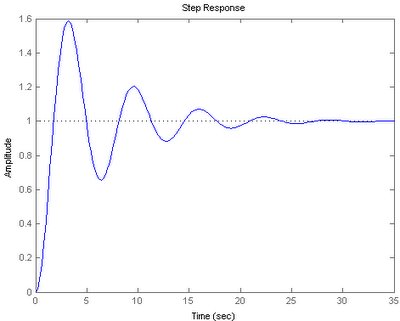
The step function only shows the step response of a system at given gain value (or controller value). For a better visualization and better view on how a controller parameters affect the step response, we could add another axis as the parameters range and see how the response of a system affected by the parameters.

1. Creating a transfer function

G = tf(1,[3 1 0]);

2. Using "step" will only show the response in 2-D

G1 = feedback(3*G,1);
step(G1);



3. In order to have 3-D plot, we need to construct the fix step for the t vector, this is due to the "Step" function will use the variable step for vector t.

t = 0:0.1:20;
u = ones(1,length(t));

4. Evaluate the gain values from 1 to 10 and plot the response in 3-D, so we can see how Kp affects the system behavior

for Kp = 1:10;
G1 = feedback(Kp*G,1);
Y(:,Kp) = lsim(G1,u,t);
end
Kp = 1:10;
surf(Kp,t,Y);
xlabel('Gain (Kp)');
ylabel('Time (sec)');
zlabel('Amplitude');
title('3-D View of Step Response with different Gain');