Basic Tutorial for Control System (II)

Using the transfer function from the previous section:




Let’s look into how to view the response of the system.

Assuming you have created a transfer function object name 'G', if you haven't, please goto Basic Tutorial for Control System (I) .

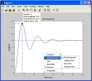
>> step(G);

Try to right click on the graph and see what information you will get from the context menu!

For arbitrary input, you could generate the input signal (time and the input) and use the "lsim" function to see the response to the input.

One thing you need to take notes is that the "time space" for the step function is not at fixed step by default.

>> [y,t,x]=step(G);

Examine the t, you would find the t is not spaced evenly.

If you would like to have the evenly spaced time samples, you need to supply the time vection in the step function. This is useful when you want to plot the 3-D View of Step Response with Different Gains.

>> [y,t,x]=step(G,0:0.25:35);

For the older version of MATLAB, you might need to use the "lsim" instead of "step" to give the evenly spaced time vector.