Basic Tutorial for Control System (III)

Using the transfer function from the previous section:

The graphic user interface (GUI) come with the control system toolbox makes the learning process faster and easier.

>> sisotool(G);


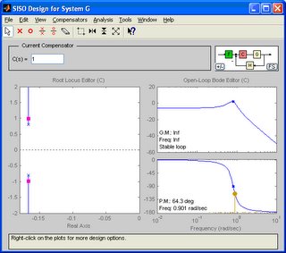
If you don’t have the transfer function object “G” yet, please refer to Basic Tutorial for Control System (I) on how to do so.


The “pink color” dot is the closed-loop poles location. Dragging the dots yield the changes of gain for the system. The good thing of this GUI is that we could view the step response updated “live” when we drag the closed-loop poles. It gives us a good view on how the changes of gain affect the system step response.

There are more things that we could do with this GUI, just explore and see it yourself!

Basic Tutorial for Control System (II)

Using the transfer function from the previous section:




Let’s look into how to view the response of the system.

Assuming you have created a transfer function object name 'G', if you haven't, please goto Basic Tutorial for Control System (I) .

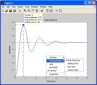
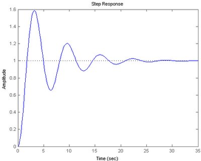
>> step(G);

Try to right click on the graph and see what information you will get from the context menu!

For arbitrary input, you could generate the input signal (time and the input) and use the "lsim" function to see the response to the input.

One thing you need to take notes is that the "time space" for the step function is not at fixed step by default.

>> [y,t,x]=step(G);

Examine the t, you would find the t is not spaced evenly.

If you would like to have the evenly spaced time samples, you need to supply the time vection in the step function. This is useful when you want to plot the 3-D View of Step Response with Different Gains.

>> [y,t,x]=step(G,0:0.25:35);

For the older version of MATLAB, you might need to use the "lsim" instead of "step" to give the evenly spaced time vector.

Basic Tutorial for Control System (I)

Let’s start with a very simple tutorial on how to create a transfer function using MATLAB and Control System Toolbox. We have a transfer function:

To create this transfer function in MATLAB, we need to understand how MATLAB create polynomial.

First, we define a variable for the numerator:
>> num = 1;

Second, we define the polynomial for the denominator:
>> den = [3 1 2];

Next, create the transfer function using the “tf” function:

>> G = tf(num, den);

How about this?




>> num = 1;
>> den = [3 0 2];

Do take note on the 0 in the middle, it must be there to represent the “missing” term for “s”.

Well, if you get error when you use “tf” command, make sure you have the control system toolbox as well. The location of a function can be location using “which” command:

>> which tf

More tutorial coming soon... :)

Useful Site for Learning Control System

A few good websites for learning control design using MATLAB:

This is the first place which I start to learn MATLAB for control design
1. Control Tutorial with MATLAB

For more details on the functions in MATLAB Control System Toolbox, the docementation is always the best place
2. Control System Toolbox Online Documentation

3-D View of Step Response with Different Gains

The step function only shows the step response of a system at given gain value (or controller value). For a better visualization and better view on how a controller parameters affect the step response, we could add another axis as the parameters range and see how the response of a system affected by the parameters.

1. Creating a transfer function

G = tf(1,[3 1 0]);

2. Using "step" will only show the response in 2-D

G1 = feedback(3*G,1);
step(G1);



3. In order to have 3-D plot, we need to construct the fix step for the t vector, this is due to the "Step" function will use the variable step for vector t.

t = 0:0.1:20;
u = ones(1,length(t));

4. Evaluate the gain values from 1 to 10 and plot the response in 3-D, so we can see how Kp affects the system behavior

for Kp = 1:10;
G1 = feedback(Kp*G,1);
Y(:,Kp) = lsim(G1,u,t);
end
Kp = 1:10;
surf(Kp,t,Y);
xlabel('Gain (Kp)');
ylabel('Time (sec)');
zlabel('Amplitude');
title('3-D View of Step Response with different Gain');

Contents by Date

Under Construction